Introduction

R and SPSS (Statistical Package for the Social Sciences) are two popular software programs for statistical analysis. There are many times when people have to move data between the two programs. For example, a program evaluator may be more familiar with cleaning data in SPSS but also requires a statistical technique that is available in R but not in her version of SPSS. 

There are different ways to import an SPSS file into R. In this tutorial, I will show you how to get an SPSS file into R using an R package called `haven`.

The Setup

This tutorial was carried out in R, version 4.3.1, version 2.5.3 of the haven package, and RStudio version 2023.06.1+524  on a Windows computer. 

Resources 

To help you follow along on your computer:

• The dataset for this tutorial is in this drive. 
• The entire code is here in this drive. 
• And a video tutorial is on YouTube.

Step 1: Install the haven Package 

The haven package is an R package that enables R to read in and write out different data formats like SAS, SPSS and Stata. Since this is the package we need to read in the SPSS data file, it is important to have it in our R environment.

If the haven package isn’t installed, it can be installed by using the install.packages() function for installing packages. This function simply takes the package name as an argument.

install.packages(“haven”)

Then, to be able to use the package, load the package using the following:

library(haven)

Note: haven is part of the tidyverse package and if tidyverse is installed then there is no need to install haven separately.

Step 2: Import and read the data file

Import the dataset into R. 

Next, read the file using read_sav() function. read_sav() is a function from the haven package. It allows you to read in .sav and .zsav files – both of which are extensions for SPSS files. 

demoData <- haven::read_sav(file = “demo.sav”)

In the code above, we assigned the variable named `demoData` to the file. This ensures the results of reading the “demo.sav” file will be saved in the object called `demoData`. 

When the data is read in, at the top right corner of the Global Environment of RStudio, we can view a summary of the dataset. 

From the RStudio tab above, we see thate the dataset `demoData` has 6,400 observations and 29 variables. 

Step 3: The structure of the dataset

To view the structure of the dataset, we need to use the `str` or structure function from the `utils` or utilities package. 

#look at the structure of the dataset utils::str(demoData)

Output

Interpretation of the output

From the output, we can see the different variables, their labels and attributes, all imported from SPSS. We have variables like $ age, $ marital, $ address, $ income, $ car etc. 

Each variable has a data type assigned to it. The first variable – $ age – is of a numeric data type and the first line has its first few values. 

There are different attributes for the variables (attributes have the @ signs beside them). One such attribute is the ‘label’ attribute. A label is metadata created in SPSS that gives more information or insight about the variable. For $ age, the label is ‘Age in years’. And so this label suggests that the values for age are in years. 

The next variable $ marital whose label reads as  ‘Marital status’ has values stored in 0s and 1s. The meaning of these values may not be intuitive to a reader. However, the variable $ marital also has an attribute called @ labels which indicates that the values of 0 and 1 have been assigned the labels ‘unmarried’ and ‘married’ respectively. 

Step 4: Viewing the head of the data

Now that we know what the structure of the data looks like, we can view the first few rows of the dataset using the head function from the utils package. 

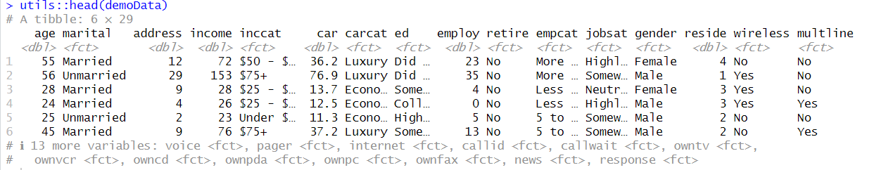
#look at the first few rows of the data utils::head(demoData)

Output

Applying the head function to the dataset demoData produced the first six rows of the dataset. From the output above, we see that the variables are now column names and the values and attributes are written in rows. 

We have age and the values for it. For marital, we see 0s and 1s and their corresponding label beside them. 

Step 5: Converting the label to factors

As mentioned above, to a reader, numeric values assigned to non-numeric variables may not make much sense. To avoid confusion we can replace the numeric values with their corresponding labels (when they exist for that variable). For example, instead of having numeric values of 0 and 1 for the variable $ marital, we can display these values as ‘unmarried’ and ‘married’. 

To make this conversion, we will apply the as_factor() function from the haven package to the entire dataset. The as_factor() function will convert variables with labels to factors, while treating the labels as the values for that variable. 

#convert variables with variable labels to factors demoData <- haven::as_factor(demoData)

Output

The new table – in contrast to the old one – shows that the numeric labels attached to the marital column and the other columns are gone. Instead, these numeric values have been replaced by their corresponding labels. 

Conclusion

In this tutorial, we have learned how to import an SPSS file into R, and how to understand the structure of the data, the attributes and labels. We also learned how to convert labeled columns into factors that have the labels as their values. 

There are still many things we can do with data imported from SPSS like using the variable labels (e.g., the actual question posed in a survey rather than simply having a variable name like question1) for reporting. Techniques such as this will be described in another blog post.

Call to Action

Are you a program evaluator or consultant that wants an easier way to leverage data analysis for your clients? Parsimony helps program evaluators and other consultants deliver clear and concise impact analysis, survey analysis, and descriptive analysis for their clients. Set up a call with Parsimony at https://parsimonyinc.com/contact/ to learn more.

Watch the video

Click here to follow along with a video showing how to import SPSS data into R.